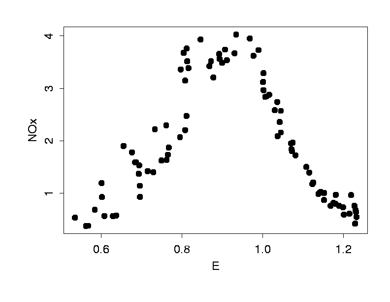

We will now show an example of a backprop network as it learns to model the highly nonlinear data we encountered before.

![]()

The left hand panel shows the data to be modeled. The right hand panel shows a network with two hidden units, each with a tanh nonlinear activation function. The output unit computes a linear combination of the two functions
 |
(1) |
Where
 |
(2) |
and
 |
(3) |
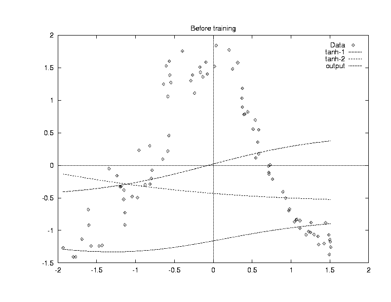
To begin with, we set the weights, a..g, to random initial values in the range [-1,1]. Each hidden unit is thus computing a random tanh function. The next figure shows the initial two activation functions and the output of the network, which is their sum plus a negative constant. (If you have difficulty making out the line types, the top two curves are the tanh functions, the one at the bottom is the network output).
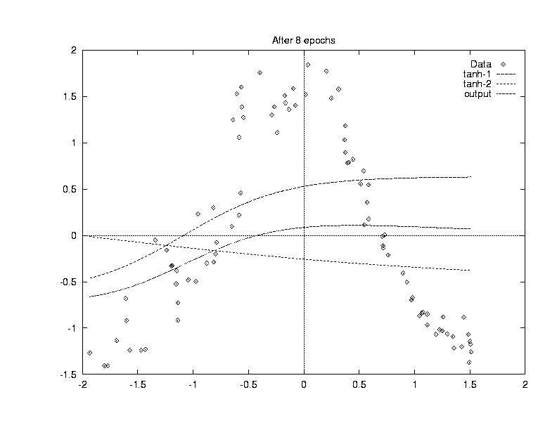
We now train the network (learning rate 0.3), updating the weights after each pattern (online learning). After we have been through the entire dataset 10 times (10 training epochs), the functions computed look like this (the output is the middle curve):
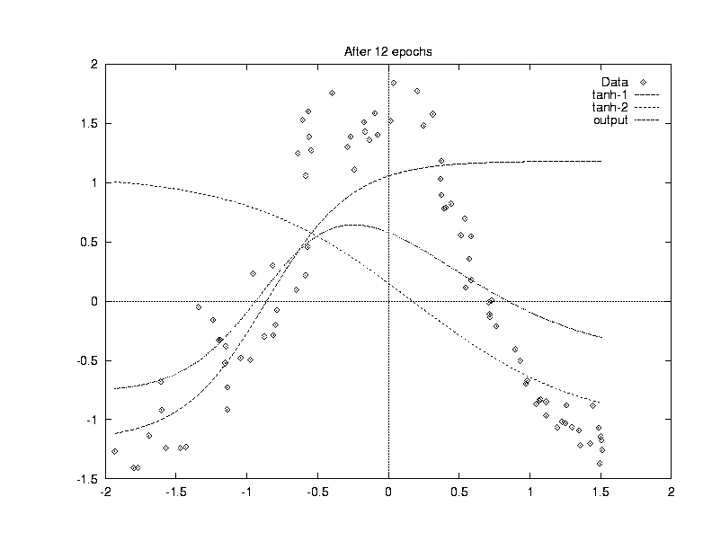
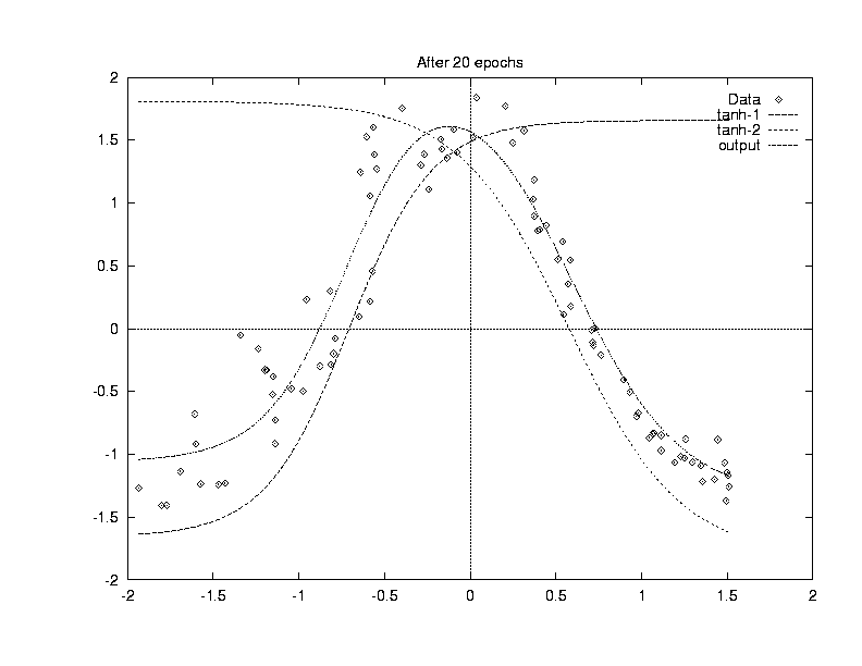
After 20 epochs, we have (output is the humpbacked curve):
and after 27 epochs we have a pretty good fit to the data:
As the activation functions are stretched, scaled and shifted by the changing weights, we hope that the error of the model is dropping. In the next figure we plot the total sum squared error over all 88 patterns of the data as a function of training epoch. Four training runs are shown, with different weight initialization each time:
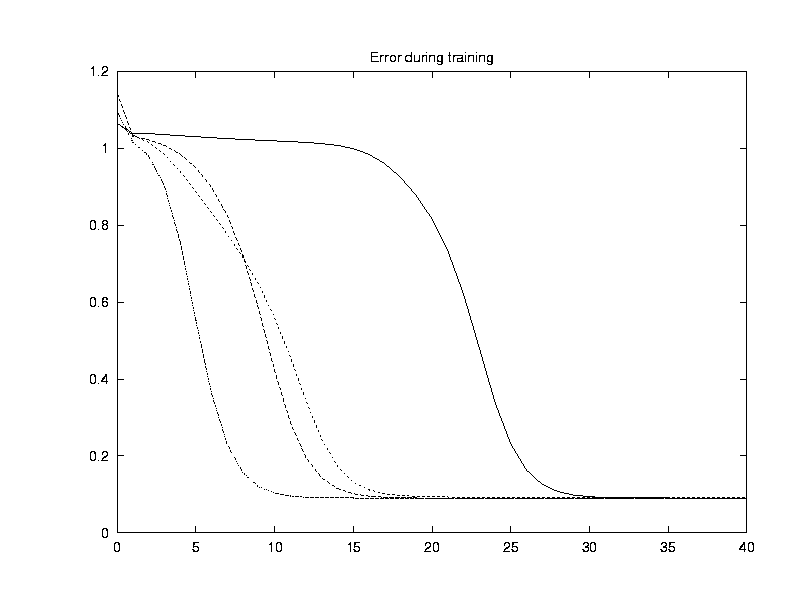
You can see that the path to the solution differs each time, both because we start from a different point in weight space, and because the order in which patterns are presented is random. Nonetheless, all training curves go down monotonically, and all reach about the same level of overall error.