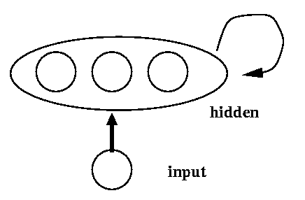
Consider the recurrent network illustrated below. A single input unit is connected to each of the three "hidden" units. Each hidden unit in turn is connected to itself and the other hidden units. As in the RTRL derivation, we do not distinguish now between hidden and output units. Any activation which enters the network through the input node can flow around from one unit to the other, potentially forever. Weights less than 1.0 will exponentially reduce the activation, weights larger than 1.0 will cause it to increase. The non-linear activation functions of the hidden units will hopefully prevent it from growing without bound.
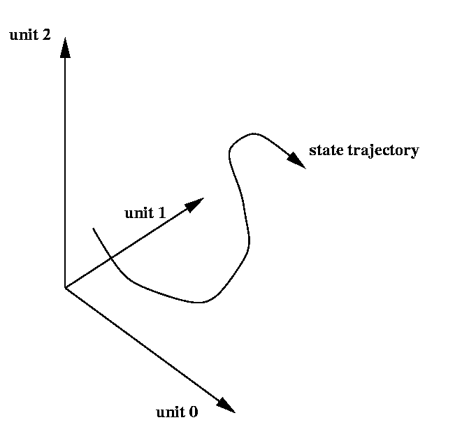
As we have three hidden units, their activation at any given time t describes a point in a 3-dimensional state space. We can visualize the temporal evolution of the network state by watching the state evolve over time.
In the absence of input, or in the presence of a steady-state input, a network will usually approach a fixed point attractor. Other behaviors are possible, however. Networks can be trained to oscillate in regular fashion, and chaotic behavior has also been observed. The development of architectures and algorithms to generate specific forms of dynamic behavior is still an active research area.
The simple recurrent network computed a gradient based on the present state of the network and its state one time step ago. Using Back Prop Through Time, we could compute a gradient based on some finite n time steps of network operation. RTRL provided a way of computing the true gradient based on the complete network history from time 0 to the present. Is this perfection?
Unfortunately not. With feedforward networks which have a large number of layers, the weights which are closest to the output are the easiest to train. This is no surprise, as their contribution to the network error is direct and easily measurable. Every time we back propagate an error one layer further back, however, our estimate of the contribution of a particular weight to the observed error becomes more indirect. You can think of error flowing in the top of the network in distinct streams. Each pack propagation dilutes the error, mixing up error from distinct sources, until, far back in the network, it becomes virtually impossible to tell who is responsible for what. The error signal has become completely diluted.
With RTRL and BPTT we face a similar problem. Error is now propagated back in time, but each time step is exactly equivalent to propagating through an additional layer of a feed forward network. The result, of course, is that it becomes very difficult to assess the importance of the network state at times which lie far back in the past. Typically, gradient based networks cannot reliably use information which lies more than about 10 time steps in the past. If you now imagine an attempt to use a recurrent neural network in a real life situation, e.g. monitoring an industrial process, where data are presented as a time series at some realistic sampling rate (say 100 Hz), it becomes clear that these networks are of limited use. The next section shows a recent model which tries to address this problem.