The neural network modeler is faced with a huge array of models and training regimes from which to select. This course can only serve to introduce you to the most common and general models. However, even after deciding, for example, to train a simple feed forward network, using some specific form of gradient descent, with tanh nodes in a single hidden layer, an important question to be addressed is remains: how big a network should we choose? How many hidden units, or, relatedly, how many weights?
By way of an example, the nonlinear data which formed our first example can be fitted very well using 40 tanh functions. Learning with 40 hidden units is considerably harder than learning with 2, and takes significantly longer. The resulting fit is no better (as measured by the sum squared error) than the 2-unit model.
The most usual answer is not necessarily the best: we guess an appropriate number (as we did above).
Another common solution is to try out several network sizes, and select the most promising. Neither of these methods is very principled.
Two more rigorous classes of methods are available, however. We can either start with a network which we know to be too small, and iteratively add units and weights, or we can train an oversized network and remove units/weights from the final network. We will look briefly at each of these approaches.
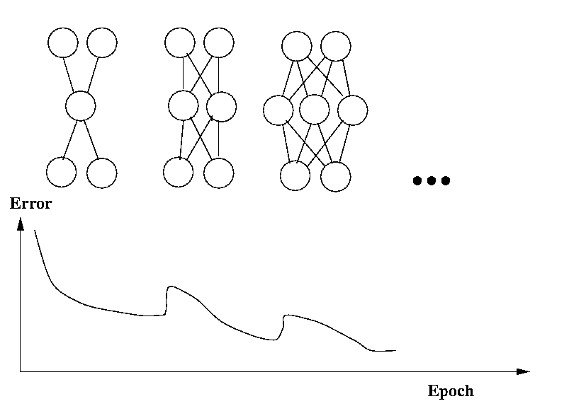
The simplest form of network growing algorithm starts with a small network, say one with only a single hidden unit. The network is trained until the improvement in the error over one epoch falls below some threshold. We then add an additional hidden unit, with weights from inputs and to outputs. We initialize the new weights randomly and resume training. The process continues until no significant gain is achieved by adding an extra unit. The process is illustrated below.

Beyond simply having too many parameters (danger of overfitting), there is a problem with large networks which has been called the herd effect. Imagine we have a task which is essentially decomposable into two sub-tasks A and B. We have a number of hidden units and randomly weighted connections. If task A is responsible for most of the error signal arriving at the hidden units, there will be a tendency for all units to simultaneously try to solve A. Once the error attributable to A has been reduced, error from subtask B will predominate, and all units will now try to solve that, leading to an increase again in the error from A. Eventually, due mainly to the randomness in the weight initialization, the herd will split and different units will address different sub-problems, but this may take considerable time.
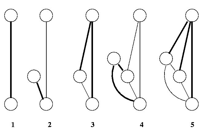
To get around this problem, Fahlman (1991) proposed an algorithm called cascade correlation which begins with a minimal network having just input and output units. Training a single layer requires no back-propagation of error and can be done very efficiently. At some point further training will not produce much improvement. If network performance is satisfactory, training can be stopped. If not, there must be some remaining error which we wish to reduce some more. This is done by adding a new hidden unit to the network, as described in the next paragraph. The new unit is added, its input weights are frozen (i.e. they will no longer be changed) and all output weights are once again trained. This is repeated until the error is small enough (or until we give up).
To add a hidden unit,we begin with a candidate unit and provide it with incoming connections from the input units and from all existing hidden units. We do not yet give it any outgoing connections. The new unit's input weights are trained by a process similar to gradient descent. Specifically, we seek to maximize the covariance between v, the new unit's value, and Eo, the output error at output unit o.
We define S as:
 |
(1) |
 are the mean values of v and Eo
over all patterns. Performing gradient ascent on the partial
derivative
  (we will
skip the explicit formula here) ensures that we end up with a unit
whose activation is maximally correlated (positively or negatively)
with the remaining error. Once we have maximized S, we freeze
the input weights, and install the unit in the network as described
above. The whole process is illustrated below.
In (1) we train the weights from input to output. In (2), we add a candidate unit and train its weights to maximize the correlation with the error. In (3) we retrain the output layer, (4) we train the input weights for another hidden unit, (5) retrain the output layer, etc. Because we train only one layer at a time, training is very quick. What is more, because the weights feeding into each hidden unit do not change once the unit has been added, it is possible to record and store the activations of the hidden units for each pattern, and reuse these values without recomputation in later epochs.

An alternative approach to growing networks is to start with a relatively large network and then remove weights so as to arrive at an optimal network architecture. The usual procedure is as follows:
Deciding which are the least important weights is a difficult issue for which several heuristic approaches are possible. We can estimate the amount by which the error function E changes for a small change in each weight. The computational form for this estimate would take us a little too far here. Various forms of this technique have been called optimal brain damage, and optimal brain surgeon.