 (Fig.
1)
(Fig.
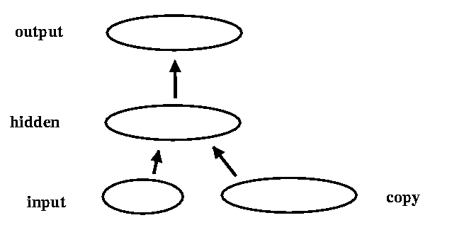
1)Consider the following two networks:
 (Fig.
1)
(Fig.
1)The network on the left is a simple feed forward network of the kind we have already met. The right hand network has an additional connection from the hidden unit to itself. What difference could this little weight make?
Each time a pattern is presented, the unit computes its activation just as in a feed forward network. However its net input now contains a term which reflects the state of the network (the hidden unit activation) before the pattern was seen. When we present subsequent patterns, the hidden and output units' states will be a function of everything the network has seen so far. The network has a sense of history, and we must think of pattern presentation as it happens in time.
 , we had to know the errors of all units in its
anterior set, Ai.
For an arbitrary unit in a recurrent network, we now define its activation at time t as:
At each time step, therefore, activation propagates forward through one layer of connections only. Once some level of activation is present in the network, it will continue to flow around the units, even in the absence of any new input whatsoever. We can now present the network with a time series of inputs, and require that it produce an output based on this series. This presents a whole set of new problems which can be addressed by the networks, as well as some rather difficult matters concerning training.
Before we address the new issues in training and operation of recurrent neural networks, let us first look at some sample tasks which have been attempted (or solved) by such networks.
Given a set of strings S, each composed of a series of symbols, identify the strings which belong to a language L. A simple example: L = {an,bn} is the language composed of strings of any number of a's, followed by the same number of b's. Strings belonging to the language include aaabbb, ab, aaaaaabbbbbb. Strings not belonging to the language include aabbb, abb, etc. A common benchmark is the language defined by the reber grammar. Strings which belong to a language L are said to be grammatical and are ungrammatical otherwise.
In some of the best speech recognition systems built so far, speech is first presented as a series of spectral slices to a recurrent network. Each output of the network represents the probability of a specific phone (speech sound, e.g. /i/, /p/, etc), given both present and recent input. The probabilities are then interpreted by a Hidden Markov Model which tries to recognize the whole utterance. Details are provided here.
A recurrent network can be trained by presenting it with the notes of a musical score. It's task is to predict the next note. Obviously this is impossible to do perfectly, but the network learns that some notes are more likely to occur in one context than another. Training, for example, on a lot of music by J. S. Bach, we can then seed the network with a musical phrase, let it predict the next note, feed this back in as input, and repeat, generating new music. Music generated in this fashion typically sounds fairly convincing at a very local scale, i.e. within a short phrase. At a larger scale, however, the compositions wander randomly from key to key, and no global coherence arises. This is an interesting area for further work.... The original work is described here.

In computing the activation, we have eliminated cycles, and so our requirement that the activations of all posterior nodes be known is met. Likewise, in computing errors, all trainable weights are feed forward only, so we can apply the standard backpropagation algorithm as before. The weights from the copy layer to the hidden layer play a special role in error computation. The error signal they receive comes from the hidden units, and so depends on the error at the hidden units at time t. The activations in the hidden units, however, are just the activation of the hidden units at time t-1. Thus, in training, we are considering a gradient of an error function which is determined by the activations at the present and the previous time steps.
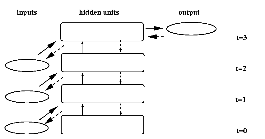
A generalization of this approach is to copy the input and hidden unit activations for a number of previous timesteps. The more context (copy layers) we maintain, the more history we are explicitly including in our gradient computation. This approach has become known as Back Propagation Through Time. It can be seen as an approximation to the ideal of computing a gradient which takes into consideration not just the most recent inputs, but all inputs seen so far by the network. The figure below illustrates one version of the process:
The inputs and hidden unit activations at the last three time steps are stored. The solid arrows show how each set of activations is determined from the input and hidden unit activations on the previous time step. A backward pass, illustrated by the dashed arrows, is performed to determine separate values of delta (the error of a unit with respect to its net input) for each unit and each time step separately. Because each earlier layer is a copy of the layer one level up, we introduce the new constraint that the weights at each level be identical. Then the partial derivative of the negative error with respect to wi,j is simply the sum of the partials calculated for the copy of wi,j between each two layers.

Elman networks and their generalization, Back Propagation Through Time, both seek to approximate the computation of a gradient based on all past inputs, while retaining the standard back prop algorithm. In the next section we will see how we can compute the true temporal gradient using a method known as Real Time Recurrent Learning.